Machine learning is a hot topic in research and industry, with new methodologies developed all the time. The speed and complexity of the field makes keeping up with new techniques difficult even for experts and potentially overwhelming for beginners.
To demystify machine learning let’s look at ten different methods, including simple descriptions, visualizations, and examples for each one.
What is Machine Learning:
The purpose of machine learning is to discover patterns in your data and then make predictions based on those often, complex patterns to answer business questions, and help solve problems. For example, if an online retailer wants to anticipate sales for the next quarter, they might use a machine learning algorithm that predicts those sales based on past sales and other relevant data. Similarly, a windmill manufacturer might visually monitor important equipment and feed the video data through algorithms trained to identify dangerous cracks.
Broadly, there are 3 types of Machine Learning Algorithms
1. Supervised Learning
This algorithm consist of a target / outcome variable (or dependent variable) which is to be predicted from a given set of predictors (independent variables). Using these set of variables, we generate a function that map inputs to desired outputs. The training process continues until the model achieves a desired level of accuracy on the training data. Examples of Supervised Learning: Regression, Decision Tree,Random Forest,KNN Logistic Regression etc.
2. Unsupervised Learning
In this algorithm, we do not have any target or outcome variable to predict / estimate. It is used for clustering population in different groups, which is widely used for segmenting customers in different groups for specific intervention. Examples of Unsupervised Learning: K-means algorithm.
3. Reinforcement Learning:
Using this algorithm, the machine is trained to make specific decisions. It works this way: the machine is exposed to an environment where it trains itself continually using trial and error. This machine learns from past experience and tries to capture the best possible knowledge to make accurate business decisions. Example of Reinforcement Learning: Markov Decision Process
List of Common Machine Learning Algorithms
Here is the list of commonly used machine learning algorithms. These algorithms can be applied to almost any data problem:
- Linear Regression
- Logistic Regression
- Decision Tree
- SVM (Support Vector Machine)
- Naive Bayes
- kNN (K-Nearest Neighbour)
- K-Means
- Random Forest
- Dimensionality Reduction Algorithms
1. Linear Regression
It is used to estimate real values (cost of houses, number of calls, total sales etc.) based on continuous variables. Here, we establish relationship between independent and dependent variables. This is represented by a linear equation Y= a *X + b.
The best way to understand linear regression is: For Example Let us say, you ask a child in fifth grade to arrange people in his class by increasing order of weight, without asking them their weights! What do you think the child will do? He / she would likely look (visually analyze) at the height and build of people and arrange them using a combination of these visible parameters. This is linear regression in real life! The child has actually figured out that height and build would be correlated to the weight by a relationship, which looks like the equation above.
In this equation:
- Y – Dependent Variable
- a – Slope
- X – Independent variable
- b – Intercept
These coefficients a and b are derived based on minimizing the sum of squared difference of distance between data points and regression line.

2. Logistic Regression
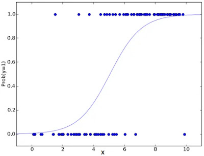
It is a classification not a regression algorithm. It is used to estimate discrete values ( Binary values like 0/1, yes/no, true/false ) based on given set of independent variables. In simple words, it predicts the probability of occurrence of an event by fitting data to a Logit function. Hence, it is also known as logit regression. Since, it predicts the probability, its output values lies between 0 and 1.
Again, let us try and understand this through a simple example.
Let’s say your friend gives you a puzzle to solve. There are only 2 outcome scenarios – either you solve it or you don’t. Now imagine, that you are being given wide range of puzzles / quizzes in an attempt to understand which subjects you are good at. The outcome to this study would be something like this – if you are given a trigonometry based tenth grade problem, you are 70% likely to solve it. On the other hand, if it is grade fifth history question, the probability of getting an answer is only 30%. This is what Logistic Regression provides you.
Coming to the math, the log odds of the outcome is modeled as a linear combination of the predictor variables.
odds= p/ (1-p) = probability of event occurrence / probability of not event occurrenceln(odds) = ln(p/(1-p))logit(p) = ln(p/(1-p)) = b0+b1X1+b2X2+b3X3....+bkXk
Above, p is the probability of presence of the characteristic of interest. It chooses parameters that maximize the likelihood of observing the sample values rather than that minimize the sum of squared errors (like in ordinary regression).
3. Decision Tree
Decision tree is a type of supervised learning algorithm that is mostly used in classification problems. It works for both categorical and continuous input and output variables. In this technique, we split the population or sample into two or more homogeneous sets based on most significant splitter / differentiator in input variables.
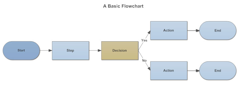
- One simple example of a Decision Tree as seen below.
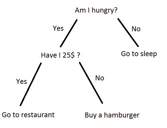
The top-most item, in this example, “Am I hungry?” is called the root. It’s where everything starts from. Branches are what we call each line. A leaf is everything that isn’t the root or a branch.
4. SVM (Support Vector Machine)
It is a classification method. In this algorithm, we plot each data item as a point in n-dimensional space (where n is number of features you have) with the value of each feature being the value of a particular coordinate.
Now, we will find some line that splits the data between the two differently classified groups of data. This will be the line such that the distances from the closest point in each of the two groups will be farthest away.
In the example shown above, the line which splits the data into two differently classified groups is the black line, since the two closest points are the farthest apart from the line. This line is our classifier. Then, depending on where the testing data lands on either side of the line, that’s what class we can classify the new data as.
5. Naive Bayes
Naive Bayes classifiers are a collection of classification algorithms based on Bayes’ Theorem. It is not a single algorithm but a family of algorithms where all of them share a common principle, i.e. every pair of features being classified is independent of each other.
Naive Bayesian model is easy to build and particularly useful for very large data sets. Along with simplicity, Naive Bayes is known to outperform even highly sophisticated classification methods.
Bayes theorem provides a way of calculating posterior probability P(c|x) from P(c), P(x) and P(x|c). Look at the equation below:
Here,
- P(c|x) is the posterior probability of class (target) given predictor (attribute).
- P(c) is the prior probability of class.
- P(x|c) is the likelihood which is the probability of predictor given class.
- P(x) is the prior probability of predictor.
6. kNN (k- Nearest Neighbors)
K-Nearest Neighbors is one of the most basic yet essential classification algorithms in Machine Learning. It belongs to the supervised learning domain and finds intense application in pattern recognition, data mining and intrusion detection.
It is widely disposable in real-life scenarios since it is non-parametric, meaning, it does not make any underlying assumptions about the distribution of data.
Example:
The following is an example to understand the concept of K and working of KNN algorithm.
Suppose we have a data set which can be plotted as follows:
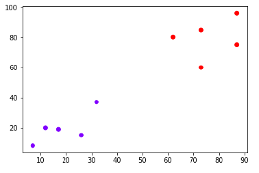
Now, we need to classify new data point with black dot (at point 60,60) into blue or red class. We are assuming K = 3 i.e. it would find three nearest data points. It is shown in the next diagram.
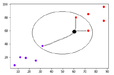
We can see in the above diagram the three nearest neighbors of the data point with black dot. Among those three, two of them lies in Red class hence the black dot will also be assigned in red class.
7. K-Means
K-means clustering is a simple unsupervised learning algorithm that is used to solve clustering problems. It follows a simple procedure of classifying a given data set into a number of clusters, defined by the letter "k," which is fixed beforehand. The clusters are then positioned as points and all observations or data points are associated with the nearest cluster, computed, adjusted and then the process starts over using the new adjustments until a desired result is reached.
K-means clustering has uses in search engines, market segmentation, statistics and even astronomy.
It is used mainly in statistics and can be applied to almost any branch of study. For example, in marketing, it can be used to group different demographics of people into simple groups that make it easier for marketers to target. Astronomers use it to shift through huge amounts of astronomical data; since they cannot analyze each object one by one, they need a way to statistically find points of interest for observation and investigation.
The algorithm:
- K points are placed into the object data space representing the initial group of centroids.
- Each object or data point is assigned into the closest k.
- After all objects are assigned, the positions of the k centroids are recalculated.
- Steps 2 and 3 are repeated until the positions of the centroids no longer move.

A Simple example of K-Means
8. Random Forest
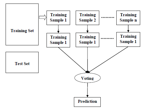
Random forest is a supervised learning algorithm which is used for both classification as well as regression. But however, it is mainly used for classification problems. As we know that a forest is made up of trees and more trees means more robust forest. Similarly, random forest algorithm creates decision trees on data samples and then gets the prediction from each of them and finally selects the best solution by means of voting. It is an ensemble method which is better than a single decision tree because it reduces the over-fitting by averaging the result.
Working of Random Forest Algorithm:
We can understand the working of Random Forest algorithm with the help of following steps −
- Step 1 − First, start with the selection of random samples from a given data set.
- Step 2 − Next, this algorithm will construct a decision tree for every sample. Then it will get the prediction result from every decision tree.
- Step 3 − In this step, voting will be performed for every predicted result.
- Step 4 − At last, select the most voted prediction result as the final prediction result.
The following diagram will illustrate its working:
9. Dimensionality Reduction Algorithms
Dimensionality reduction is a series of techniques in machine learning and statistics to reduce the number of random variables to consider. It involves feature selection and feature extraction. Dimensionality reduction makes analyzing data much easier and faster for machine learning algorithms without extraneous variables to process, making machine learning algorithms faster and simpler in turn.
Dimensionality reduction attempts to reduce the number of random variables in data. A K-nearest-neighbors approach is often used. Dimensionality reduction techniques are divided into two major categories: feature selection and feature extraction.
Feature selection techniques find a smaller subset of a many-dimensional data set to create a data model. The major strategies for feature set are filter, wrapper (using a predictive model) and embedded, which perform feature selection while building a model.
Feature extraction involves transforming high-dimensional data into spaces of fewer dimensions. Methods include principal component analysis, kernel PCA, graph-based kernel PCA, linear discriminant analysis and generalized discriminant analysis.
Future Scope :
Machine Learning is currently one of the hottest topics in IT.. Technologies such as digital, big data, Artificial Intelligence, automation and machine learning are increasingly shaping future of work and jobs is a specific set of techniques that enable machines to learn from data, and make predictions. When the biases of our past and present fuel the predictions of the future, it's a tall order to expect AI to operate independently of human flaws.
Summary:
I’ve tried to cover the nine most important machine learning methods: from the most basic to the bleeding edge. Studying these methods well and fully understanding the basics of each one can serve as a solid starting point for further study of more advanced algorithms and methods.



No comments:
Post a Comment